Forecast the Family, Split by the Curve
In footwear, the item a buyer orders — one style, one colourway, one size, one width — is the item with the least data behind it. A single UPC often sells two pairs in nine months: not a pattern, just noise. buffers.ai forecasts where the demand is readable — the style family — and then splits that forecast down to every colourway, size, and width using a size curve learned from the store's own sales. The same curve is what lets a new SKU be ordered before it has sold a single pair.
The SKU You Buy Is the SKU You Can't Forecast
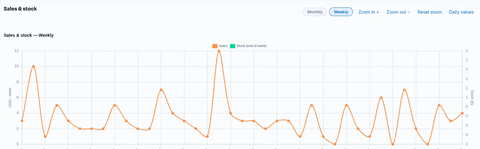
Here is what nine months of sales looks like at one specialty running-footwear store. Every forecasting model — statistical or machine learning — needs repeated observations to find a level, a trend, and a season. At the UPC level there are almost none: most sizes of most colourways sold once or twice, and the rest of the time sat at zero. Forecast that directly and you get either zero (and a stock-out on the first customer who asks) or a flat fraction of a pair spread across every size (and dead stock in the sizes nobody wears).
UPCs on file
Median units sold per UPC in 9 months
Of UPCs sold on fewer than 10 days
Median selling days per style family
Group the same 1,155 UPCs into 36 style families and the picture changes: a median family sold on 26 different days, and the largest sold hundreds of pairs. That is enough history to backtest a model against — and that is where the forecast belongs.
Forecast the Family, With Its Own Champion Model
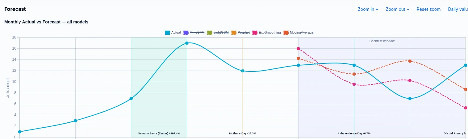
Sales are uploaded with the style family as the forecasting unit and the UPC kept alongside it, so nothing is thrown away. Each family then goes through the same process as any SKU in buffers.ai: five forecasting engines — TimesFM, LightGBM, Prophet, Exponential Smoothing, and Moving Average — are backtested against months of sales they haven't seen, and the closest fit becomes that family's champion.
Holidays and promotions measured from the store's own history are layered in, and each family orders against its own lead time — so the quantity covers the demand that will exist when the shipment lands, not the demand in the week the order is placed.
Split by Colourway, Then by Size
The family forecast is split into order lines with one multiplication:
UPC qty = family qty × P(colourway | family) × P(size, width | category, gender)
Colourway share: recent, not historical
In footwear, a new version or colourway replaces the old one rather than adding to it. So only colourways that sold within 120 days of the family's last sale are in play, each weighted by its last 90 days of units plus a small prior — enough that a colourway launched last week still gets a share before it has had time to sell.
Size curve: a property of the customers, not the shoe
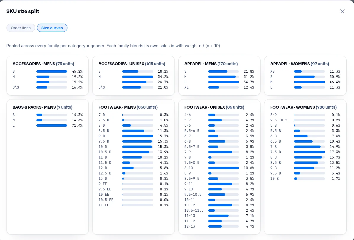
Whether a store sells more 9s or more 11s depends far more on who walks in than on which model they're buying. So the curve is pooled across every family per category × gender, with width (D, EE, B) part of each size cell, and lightly smoothed so an unsold in-between size isn't a hard zero. Each family's own sales are then blended in.
How much of a family's own curve to trust
A family's size mix is blended with the pooled curve in proportion to how much it has sold:
curve = (n · Pfamily + 10 · Ppooled) / (n + 10)
where n is the family's units sold. A best-seller with 250 pairs keeps its own shape — maybe its last runs small and customers size up. A 10-unit family is half pooled, so three stray sales can't decide its whole size run. The weight of 10 isn't a guess: on the retailer's holdout it beat both the family-only curve and heavier pooling (25, 50, 100) on every window tested.
| Family units | Own curve | Pooled curve |
|---|---|---|
| 0 (new family) | 0% | 100% |
| 10 | 50% | 50% |
| 40 | 80% | 20% |
| 250 | 96% | 4% |
Order Whole Pairs at a Service Level, Not a Rounded Average
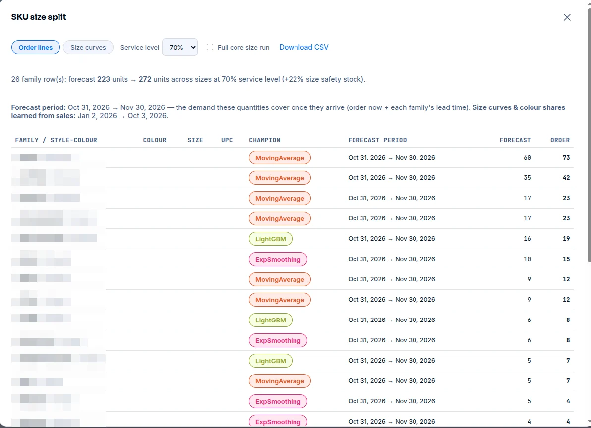
At this volume a size's expected demand is often under one pair, and plain rounding turns that into zero — exactly the size that then walks out of the store unsold. Instead, each size orders the quantity that covers its demand with the chosen probability (a Poisson quantile at 50–90% service level).
The quantile is taken per size, summed across colourways — size isn't substitutable, colour largely is. Those pairs are then dealt to colourways by recent share, so a size that needs two pairs goes to the two strongest colourways rather than a tenth of a pair to each of twenty. An optional full core size run guarantees at least one pair across the sizes that make up 80% of the curve.
Example: a 60-pair men's family forecast, split over the D-width curve above
| Size | Curve | Expected | Rounded | 70% service |
|---|---|---|---|---|
| 8 D | 4.5% | 2.7 | 3 | 3 |
| 8.5 D | 11.3% | 6.8 | 7 | 8 |
| 9 D | 15.7% | 9.4 | 9 | 11 |
| 9.5 D | 15.3% | 9.2 | 9 | 11 |
| 10 D | 15.3% | 9.2 | 9 | 11 |
| 10.5 D | 13.9% | 8.3 | 8 | 10 |
| 11 D | 10.1% | 6.1 | 6 | 7 |
| 11.5 D | 4.1% | 2.5 | 2 | 3 |
| 12 D | 5.8% | 3.5 | 3 | 4 |
| 12.5 D | 1.6% | 1.0 | 1 | 1 |
| 13 D | 0.8% | 0.5 | 0 | 1 |
| Total pairs | 57 | 70 | ||
Rounding orders 57 pairs against a 60-pair forecast and skips size 13 entirely. The 70% service level orders 70: the 10 extra pairs are the family's safety stock, spread across the sizes where a miss is most likely.
Ordering SKUs That Have Never Sold
Because the forecast lives at the family and the size mix lives in the pooled curve, a new SKU never has to start from zero. Whatever is new about it, something above it already has history.
A new version of an existing style
The family is the forecast unit, so version 9 of a running shoe inherits the demand history version 8 built. Its colourways start from the family's size curve on day one, and the old version's colourways drop out of the split once they stop selling.
A new colourway
Colourway shares come from recent sales plus a small starting allowance, so a colourway that launched last week still gets a slice of the family's order instead of zero. As it sells, its share moves to match.
A size the store has never sold
The pooled curve is smoothed along the size axis: an unsold 12.5 between a selling 12 and 13 borrows from its neighbours, so it isn't treated as zero demand just because nobody has asked for it yet.
Tested on Sales the Model Never Saw
To check the split, we fit every curve on the retailer's sales up to a cutoff, then compared each family's predicted size mix against the sizes customers actually bought afterwards — at 60-, 90-, and 120-day holdouts. Error is size-level WAPE (lower is better); fill rate is the share of holdout pairs that landed on a size the split would have stocked.
| Holdout | Pairs sold | Pooled + family (used) | Family only | Pooled only | Flat across sizes | Fill rate |
|---|---|---|---|---|---|---|
| 60 days | 441 | 59.0% | 60.3% | 64.2% | 97.1% | 93.2% |
| 90 days | 782 | 46.2% | 46.6% | 50.4% | 83.9% | 91.6% |
| 120 days | 1,173 | 48.1% | 49.8% | 49.4% | 78.9% | 92.8% |
Best on every window
The blended curve beat the family's own curve, the pooled curve, and a flat split at 60, 90, and 120 days.
39–45% less error than flat
Spreading an order evenly across sizes — the default when there's no curve — is the worst option by a wide margin.
92–93% of pairs had a size waiting
Nearly every customer in the holdout bought a size the split would have put on the shelf.
Why is size-level error still in the 46–59% range? Because at two pairs per UPC, much of what's left is pure chance — which of three customers this month happened to wear a 10.5. No curve can predict that; what it can do is make sure the size is there when they come in, which is what the fill rate measures.
Family forecasting forecasts demand at the level where a product's sales are dense enough to model — the style family — and allocates it down to SKUs with learned proportions: here, a recency-weighted colourway share and a size × width curve pooled across the category and shrunk toward each family's own history. It's how buffers.ai plans footwear and apparel assortments where most individual SKUs sell too rarely to forecast on their own.
Read next: How buffers.ai chooses the best forecast · The Monthly Buy Plan · Forecasting module
See the size curves in your own sales
Send us a sales file with style, colour, and size, and we'll show you your pooled size curves and a size-level order for your next buy — built on your own data.